Here is the R script for analyzing the tutorial dataset:

library(openintro)
library(ggplot2)

data("tourism", package = 'openintro') # Question 8.21

ggplot(tourism, aes(x = visitor_count_tho)) +
    geom_histogram()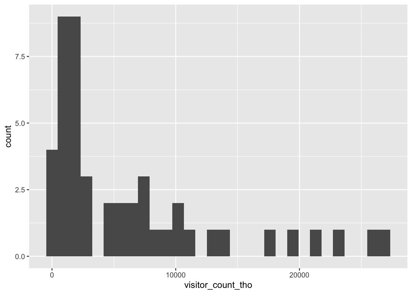

ggplot(tourism, aes(x = tourist_spending)) +
    geom_histogram()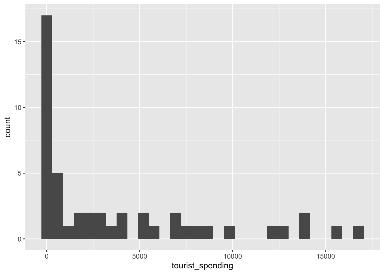

ggplot(tourism, aes(x = visitor_count_tho, y = tourist_spending)) +
    geom_point() +
    geom_smooth(method = 'lm', se = FALSE, formula = y ~ x) +
    scale_x_log10() + scale_y_log10()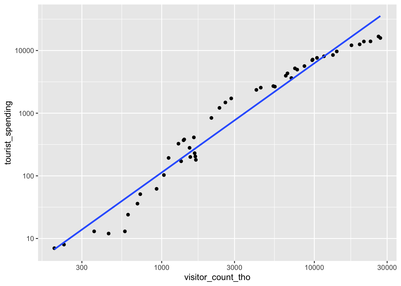

lm.out <- lm(visitor_count_tho ~ tourist_spending, data = tourism)
summary(lm.out)

## 
## Call:
## lm(formula = visitor_count_tho ~ tourist_spending, data = tourism)
## 
## Residuals:
##      Min       1Q   Median       3Q      Max 
## -1672.01  -377.84     3.28   410.00  2674.76 
## 
## Coefficients:
##                   Estimate Std. Error t value Pr(>|t|)    
## (Intercept)      636.75289  151.86868   4.193 0.000127 ***
## tourist_spending   1.49912    0.02466  60.786  < 2e-16 ***
## ---
## Signif. codes:  0 '***' 0.001 '**' 0.01 '*' 0.05 '.' 0.1 ' ' 1
## 
## Residual standard error: 815.9 on 45 degrees of freedom
## Multiple R-squared:  0.988,  Adjusted R-squared:  0.9877 
## F-statistic:  3695 on 1 and 45 DF,  p-value: < 2.2e-16

lm.out.log <- lm(log(visitor_count_tho) ~ log(tourist_spending), data = tourism)
summary(lm.out.log)

## 
## Call:
## lm(formula = log(visitor_count_tho) ~ log(tourist_spending), 
##     data = tourism)
## 
## Residuals:
##      Min       1Q   Median       3Q      Max 
## -0.49935 -0.14620 -0.01635  0.18520  0.58194 
## 
## Coefficients:
##                       Estimate Std. Error t value Pr(>|t|)    
## (Intercept)            4.36409    0.12413   35.16   <2e-16 ***
## log(tourist_spending)  0.54839    0.01755   31.25   <2e-16 ***
## ---
## Signif. codes:  0 '***' 0.001 '**' 0.01 '*' 0.05 '.' 0.1 ' ' 1
## 
## Residual standard error: 0.2813 on 45 degrees of freedom
## Multiple R-squared:  0.956,  Adjusted R-squared:  0.955 
## F-statistic: 976.9 on 1 and 45 DF,  p-value: < 2.2e-16

tourism$residual <- resid(lm.out)
tourism$residual.log <- resid(lm.out.log)

ggplot(tourism, aes(x = tourist_spending, y = residual)) +
    geom_hline(yintercept = 0) +
    geom_point()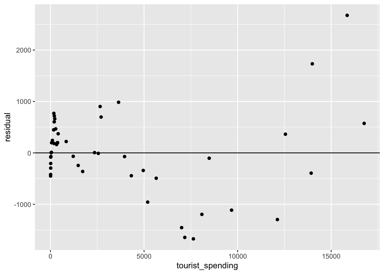

ggplot(tourism, aes(x = tourist_spending, y = residual.log)) +
    geom_hline(yintercept = 0) +
    geom_point()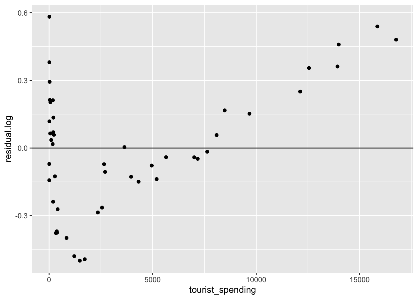

hist(tourism$residual)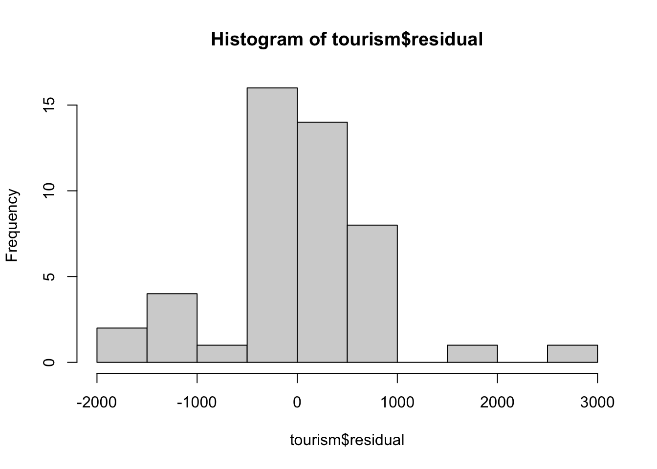

ggplot(tourism, aes(x = residual)) + geom_histogram(bins = 7)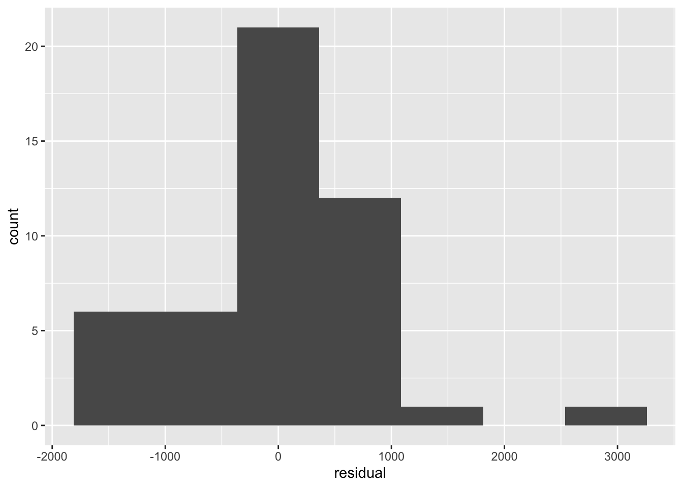

ggplot(tourism, aes(x = residual)) + geom_density()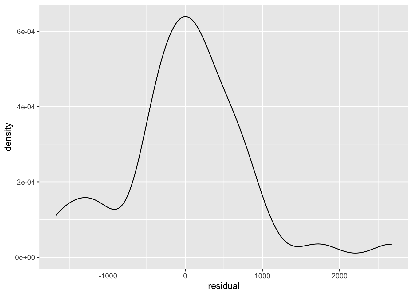

Here is the R script that looks at how the F-statistic is calculated.

poverty <- read.table("https://raw.githubusercontent.com/jbryer/DATA606Spring2021/master/course_data/poverty.txt", h = T, sep = "\t")
names(poverty) <- c("state", "metro_res", "white", "hs_grad", "poverty", "female_house")
poverty <- poverty[,c(1,5,2,3,4,6)]
head(poverty)

##        state poverty metro_res white hs_grad female_house
## 1    Alabama    14.6      55.4  71.3    79.9         14.2
## 2     Alaska     8.3      65.6  70.8    90.6         10.8
## 3    Arizona    13.3      88.2  87.7    83.8         11.1
## 4   Arkansas    18.0      52.5  81.0    80.9         12.1
## 5 California    12.8      94.4  77.5    81.1         12.6
## 6   Colorado     9.4      84.5  90.2    88.7          9.6

# Sample size
n <- nrow(poverty)
# Total variance for the outcome variable
SSy <- sum((poverty$poverty - mean(poverty$poverty))^2)

# Start with one predictor
lm.out1 <- lm(poverty ~ female_house, data = poverty)
summary(lm.out1)

## 
## Call:
## lm(formula = poverty ~ female_house, data = poverty)
## 
## Residuals:
##     Min      1Q  Median      3Q     Max 
## -5.7537 -1.8252 -0.0375  1.5565  6.3285 
## 
## Coefficients:
##              Estimate Std. Error t value Pr(>|t|)    
## (Intercept)    3.3094     1.8970   1.745   0.0873 .  
## female_house   0.6911     0.1599   4.322 7.53e-05 ***
## ---
## Signif. codes:  0 '***' 0.001 '**' 0.01 '*' 0.05 '.' 0.1 ' ' 1
## 
## Residual standard error: 2.664 on 49 degrees of freedom
## Multiple R-squared:  0.276,  Adjusted R-squared:  0.2613 
## F-statistic: 18.68 on 1 and 49 DF,  p-value: 7.534e-05

anova(lm.out1)

## Analysis of Variance Table
## 
## Response: poverty
##              Df Sum Sq Mean Sq F value    Pr(>F)    
## female_house  1 132.57 132.568  18.683 7.534e-05 ***
## Residuals    49 347.68   7.095                      
## ---
## Signif. codes:  0 '***' 0.001 '**' 0.01 '*' 0.05 '.' 0.1 ' ' 1

# Note that F-statistic is the same summary(lm.out1).
# From the ANOVA output, it is the ratio of mean square model
# (i.e. female_house here) to mean square error/residual.
132.568 / 7.095

## [1] 18.68471

# However, this only works with one predictor.
SSresid <- sum(lm.out1$residuals^2)
SSmodel <- SSy - SSresid
k <- length(lm.out1$coefficients) - 1
((SSmodel) / k) / (SSresid / (n - (k + 1)))

## [1] 18.68348

lm.out2 <- lm(poverty ~ female_house + white, data = poverty)
summary(lm.out2)

## 
## Call:
## lm(formula = poverty ~ female_house + white, data = poverty)
## 
## Residuals:
##     Min      1Q  Median      3Q     Max 
## -5.5245 -1.8526 -0.0381  1.3770  6.2689 
## 
## Coefficients:
##              Estimate Std. Error t value Pr(>|t|)    
## (Intercept)  -2.57894    5.78491  -0.446 0.657743    
## female_house  0.88689    0.24191   3.666 0.000615 ***
## white         0.04418    0.04101   1.077 0.286755    
## ---
## Signif. codes:  0 '***' 0.001 '**' 0.01 '*' 0.05 '.' 0.1 ' ' 1
## 
## Residual standard error: 2.659 on 48 degrees of freedom
## Multiple R-squared:  0.2931, Adjusted R-squared:  0.2637 
## F-statistic: 9.953 on 2 and 48 DF,  p-value: 0.0002422

anova(lm.out2)

## Analysis of Variance Table
## 
## Response: poverty
##              Df Sum Sq Mean Sq F value    Pr(>F)    
## female_house  1 132.57 132.568 18.7447 7.562e-05 ***
## white         1   8.21   8.207  1.1605    0.2868    
## Residuals    48 339.47   7.072                      
## ---
## Signif. codes:  0 '***' 0.001 '**' 0.01 '*' 0.05 '.' 0.1 ' ' 1

# How is the F-Statistic calculated
# Ho: All coefficients are zero
# Ha: At least one coefficient is nonzero
n <- nrow(poverty)
SSresid <- sum(lm.out2$residuals^2)
SSy <- sum((poverty$poverty - mean(poverty$poverty))^2)
SSmodel <- SSy - SSresid
k <- length(lm.out2$coefficients) - 1
((SSmodel) / k) / (SSresid / (n - (k + 1)))

## [1] 9.952561